KOMEC GLOBAL / COMPUTATIONAL FLUID DYNAMICS

CFD modelling
for water treatment.

SAVED CFD CONCENTRATION · 0–3,433.788 sTime compressed · fixed rendering settings
CONTACT-TANK EXAMPLE · PASSIVE-TRACER VOLUMEEngineering purpose

Green represents the computed tracer concentration in water. Fixed opacity emphasizes concentration variation; the sections below provide local concentration values. Labelled 10-second sequence

Diagnostic study. This retained run has known transport defects. These views demonstrate visualization and review methods; they do not establish physical residence time or treatment performance. Study basis

EXAMPLE / BAFFLED DISINFECTION CONTACT TANK

Computational cells
744,602
Retained concentration states
345
Simulation time represented
57.23 min
Main tank plan
18 × 8 m

WATER-QUALITY ENGINEERING

Contact-tank hydraulics
and disinfection.

A disinfection contact tank provides time for a disinfectant to act. Baffles influence the flow path and the distribution of contact times. Short-circuiting and poorly exchanged regions can make the hydraulic behaviour differ from the nominal volume divided by flow rate.

The engineering aim is to assess how the geometry and operating conditions influence hydraulic contact, then combine that evidence with disinfectant residual, reaction conditions and applicable water-quality criteria. Engineering background: US EPA guidance, Appendix C.

This example visualizes passive-tracer concentration. It does not model disinfectant decay or pathogen inactivation, and the retained run is not a validated basis for contact-time or treatment-performance estimates.

01

THE ISOSURFACES

Surfaces of equal
concentration.

The isosurfaces locate three fixed concentration levels within the saved tracer field. Their changing shape shows where those levels occur relative to the baffles and columns.

SAVED CFD CONCENTRATION · 0–3,433.788 sTime compressed · fixed rendering settings
CONCENTRATION ISOSURFACES

C/Cin = 25%, 50% and 75%. These surfaces identify concentration levels; they are not water surfaces or particle paths. The same retained simulation underlies the opening volume render and this view.
Download the labelled 10-second sequence

02

THE SECTION

Concentration
at two elevations.

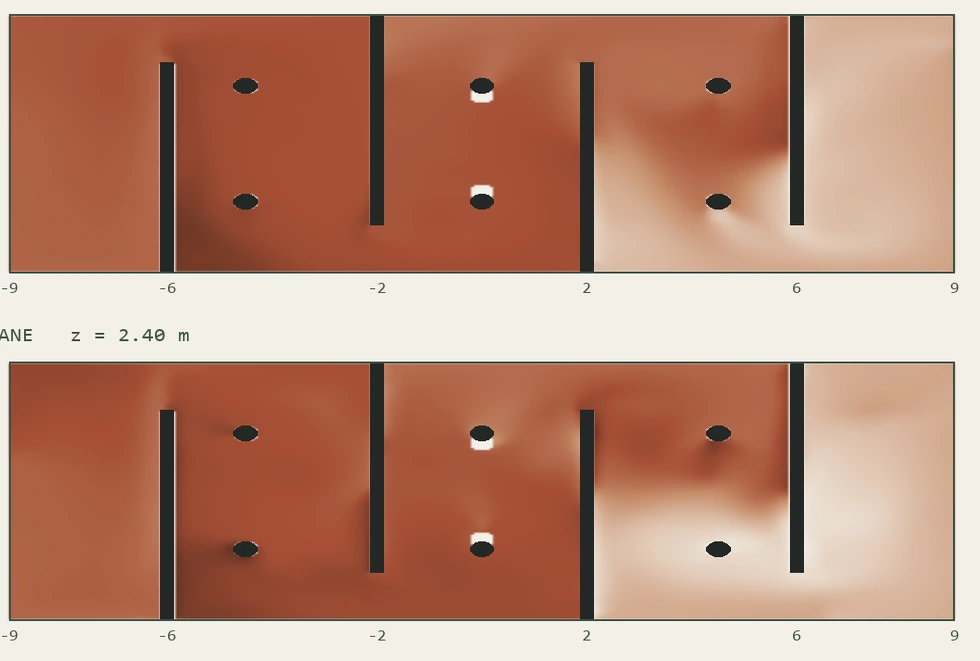
The two horizontal planes show concentration variation at the same saved simulation time. Both use the same fixed concentration scale, independently of volume opacity.

1,654.044 sSAVED SIMULATION TIME
HORIZONTAL CONCENTRATION SECTIONSt = 1,654.044 s

LOWER PLANE · z = 0.90 m

Lower horizontal concentration section at 1,654.044 simulation seconds, elevation 0.90 metres.

UPPER PLANE · z = 2.40 m

Upper horizontal concentration section at 1,654.044 simulation seconds, elevation 2.40 metres.
C/Cin

0%50%100%

Fixed concentration scale. White regions are outside the sampled water mask. Plan coordinates in metres; main tank 18 × 8 m.
03

THE CONTEXT

Baffles, columns
and concentration.

A concentration cutaway keeps the arrangement of baffles, columns and connections visible while the saved field changes.

SAVED CFD CONCENTRATION · 0–3,433.788 sTime compressed · fixed rendering settings
COPPER CURRENT

Concentration is normalized by the inlet reference Cin and displayed with a fixed colour scale. The cutaway relates the field to the contact-tank geometry.

04

THE QUANTITIES

Outlet response
and contact-time analysis.

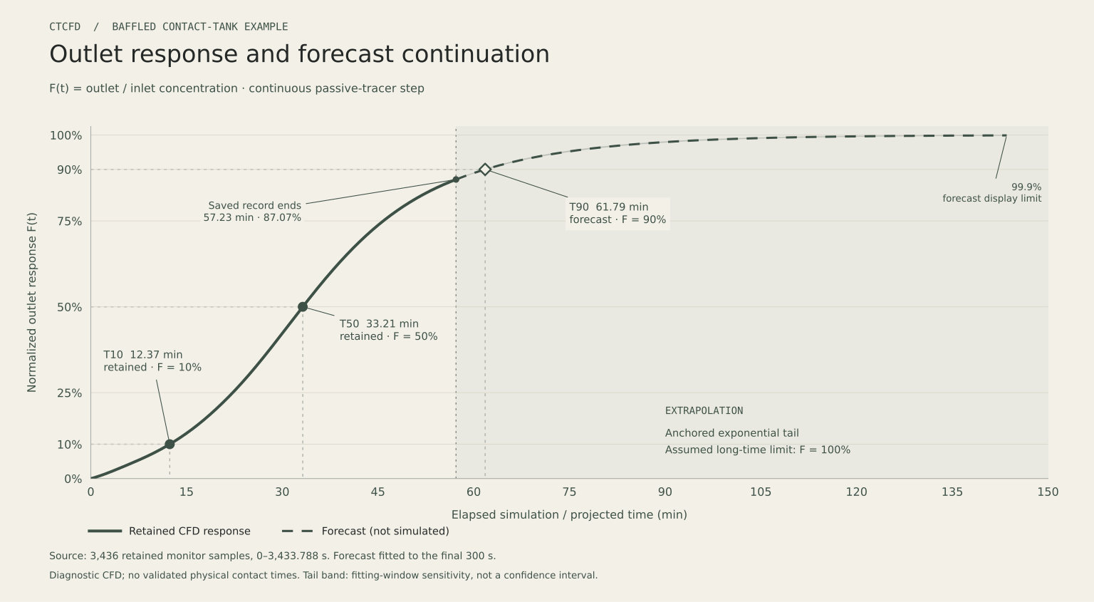
Read the T10, T50 and T90 response crossings alongside nominal hydraulic detention time. The forecast is shown separately from the retained CFD record.

T10, T50 and T90 below denote the 10%, 50% and 90% crossings of this diagnostic numerical response. They are not validated physical contact times.

T10 Retained response
12.37 min
F(t) = 10%
Interpolated between saved samples.
T50 Retained response
33.21 min
F(t) = 50%
Interpolated between saved samples.
T90 Forecast
61.79 min
F(t) = 90%
Beyond the retained simulation.
V/Q Nominal detention
38.73 min
464.78 m³ ÷ 0.200 m³/s
Reference volume and design flow.
Diagnostic outlet response F(t). T10 is 12.37 minutes and T50 is 33.21 minutes from retained samples. A dashed exponential forecast starts at 57.23 minutes and projects T90 at 61.79 minutes. These are not validated physical contact times.

The solid curve uses 3,436 retained monitor samples. The dashed curve begins at 57.23 min, where F = 87.07%, and is an exponential extrapolation. No later CFD concentration fields have been generated.

Full-size figure

READING THE RESPONSE

Crossings and
nominal detention.

The numerical outlet response reaches 10% before the nominal V/Q time and 50% at 33.21 min. At V/Q = 38.73 min, the computed outlet concentration is 62.4% of the inlet reference.

The estimated 10–90% rise interval is 49.42 min. It combines the retained T10 crossing with the forecast T90 crossing. These quantities describe the curve; the identified numerical errors prevent attributing the spread to tank hydraulics alone.

WATER-QUALITY INTERPRETATION

Contact time
and disinfection.

In a suitably qualified conservative-tracer step study, the 10% outlet response can inform the effective hydraulic contact time T10. Nominal V/Q is a separate volume-and-flow reference; it is neither T10 nor a measured mean residence time.

For disinfection assessment, CT combines an applicable disinfectant residual with a qualified contact time. This passive-tracer reference concentration is not a disinfectant residual. The present run therefore provides no defensible numerical disinfection CT or pathogen-inactivation estimate.

Method background: US EPA guidance, §4.4 and Appendix E.
Forecast assumptions and sensitivity

The continuation assumes the normalized outlet response approaches F = 1 and fits the logarithm of the remaining response, 1 − F, over the final 300 s. It is anchored to the last retained point and uses interval-duration weights.

Fforecast(t) = 1 − (1 − Fend) exp[−k(t − tend)]

Here t is in seconds, tend = 3,433.788 s, Fend = 0.870677746 and k = 9.39190 × 10⁻⁴ s⁻¹. The displayed tail stops at 99.9% at 143.52 min; it never reaches exactly 100% at a finite time under this model.

Using 150, 300, 600 and 900 s fitting windows gives T90 = 61.6961.84 min. The narrow band is fitting-window sensitivity, not a confidence interval; it excludes uncertainty in the model, asymptote and CFD solution.

A separate check withheld the final 100.7 s and fitted the preceding 300 s. Its maximum response error was 0.033 percentage points. Agreement over that short interval does not validate the long tail or overcome the run’s continuity and redistribution errors.

SPATIAL VARIATION

Concentration
distributions.

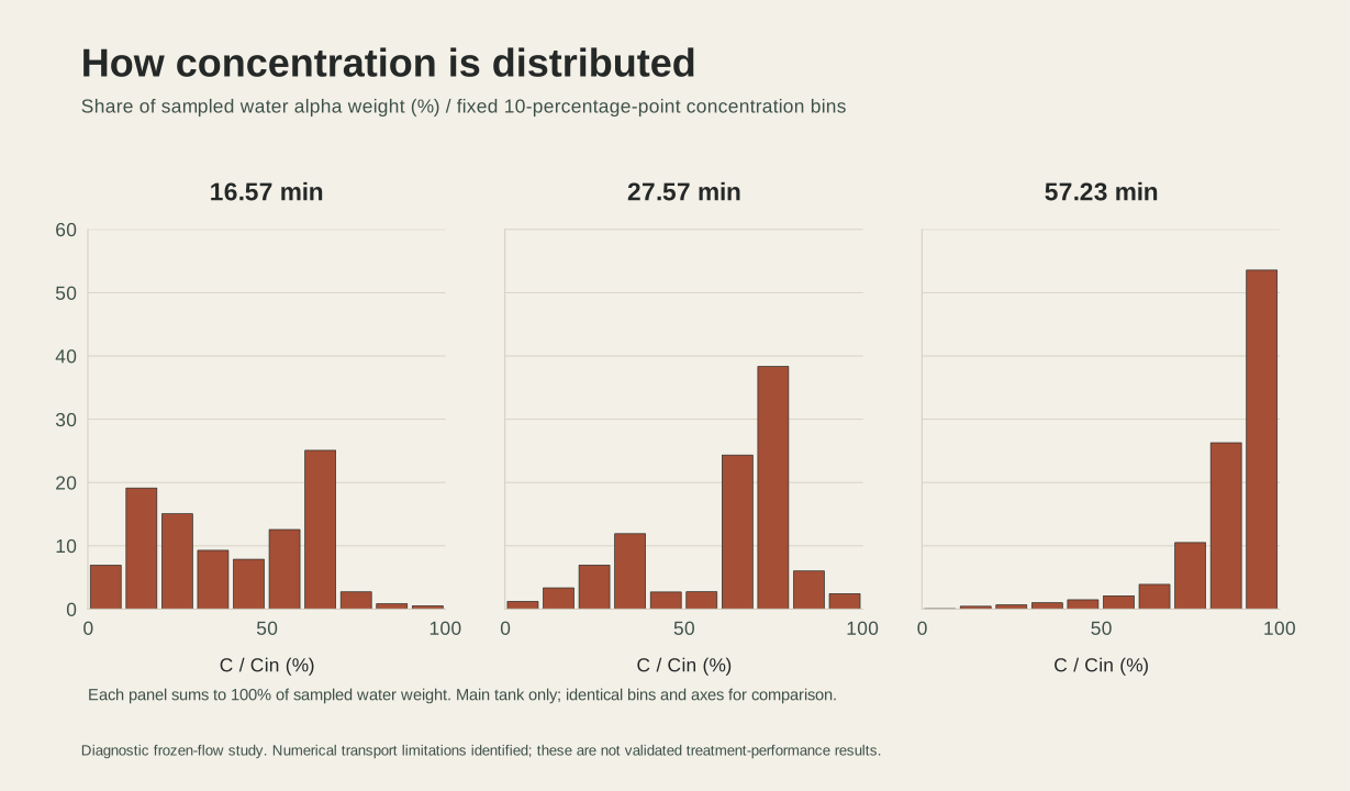
Compare the distribution across fixed concentration bins at three saved times. These water-weighted display-grid summaries make variation visible without reducing the field to one number.

Concentration distributions at three saved states, shown with identical ten-percentage-point bins and axes.

Each panel sums to 100% of sampled water weight inside the main tank. Identical bins and axes support comparison.

Full-size figure

THE ENGINEERING APPROACH

Modelling method
and numerical checks.

Frame the decision, examine the numerical evidence, then decide what the model can support.

  1. 01

    Define

    Set the geometry, operating conditions and engineering question. Record assumptions before interpreting a result.

  2. 02

    Resolve

    Review the mesh, boundary conditions, convergence and conservation. Test sensitivities appropriate to the study.

  3. 03

    Examine

    Connect spatial fields with response curves. Use sections and consistent scales to inspect variation and anomalies.

  4. 04

    Qualify

    Compare against suitable reference evidence. State uncertainty and limitations alongside any design conclusion.

STUDY BASIS / READ WITH THE FIGURES

Model assumptions
and limitations.

This is a visualization demonstration using a retained diagnostic CTCFD run. Known local continuity errors in the frozen carrier and nonlocal concentration redistribution limit physical interpretation.

Geometry
Main tank 18 × 8 m; four baffles and six columns.
Input
Continuous inlet passive-tracer step, Cin = 1 kg/m³ as a model reference concentration; design flow 0.200 m³/s.
Hydraulic basis
Frozen carrier from hydraulic time 106.375836 s.
Field record
345 saved concentration states, 0–3,433.788 s; 60 mm display grid.
Animation
10 seconds at 24 fps. The opening volume uses 216 saved states; the other views use 96 saved states, with opening and closing holds. No generated intermediate fields or particle trajectories.
How to read the views and quantities

Cloud and surfaces. Cloud opacity, viewing depth and shading affect appearance. Use sections to read local concentration. The contour view shows C/Cin = 25%, 50% and 75%, restricted to display cells whose corners all have water fraction α ≥ 0.5.

Outlet response. F(t) is the positive outgoing water-flux-weighted outlet concentration divided by Cin. It is not cumulative tracer mass recovery.

Tank average. Retained scalar inventory divided by 464.7798166 m³ reference water volume and Cin. The source inventory uses max(α, 10⁻⁸) capacity.

Spatial summaries. Compartment means and distributions use α-weighted water nodes on the 60 mm display grid within the main tank. They are not exact finite-volume integrations.

A qualified hydraulic and tracer rerun, with suitable validation, is needed before using this study for physical breakthrough, residence-time, disinfection-performance or design-improvement claims.

KOMEC GLOBAL / CFD STUDIES

CFD modelling
study enquiries.

For a CFD modelling enquiry, provide the geometry, operating conditions and engineering question. The study scope should define the required analyses, validation evidence and intended use of the results.

CFD modelling enquiry Visit KOMEC GLOBAL